Adding OpenStreetMaps To Matplotlib
Adding context to thousands of dots
Adding a map to your visuals is a great way to quickly understand the geographic information you're trying to investigate. Thankfully there are quite a few packages and libraries (like geopandas, cartopy, smopy, folium, tilemapbase, or ipyleaflet) that can make creating these visuals fairly straightforward and easy in your jupyter notebooks or whatever stack you're using.
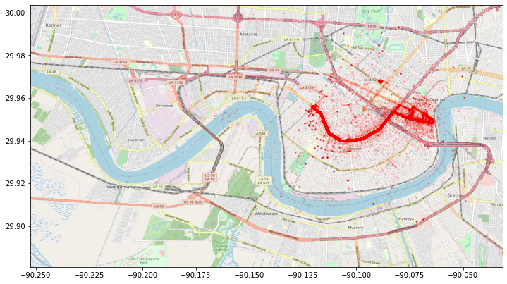
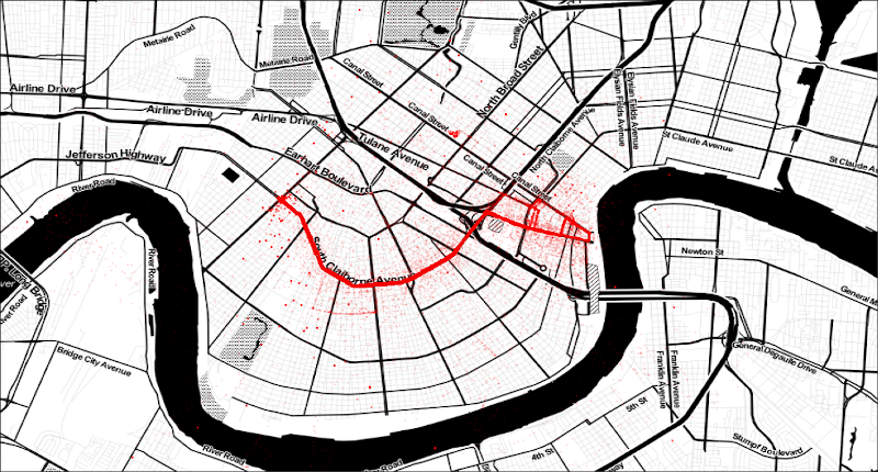
For this essay though, I'll walk through the process of adding a base-map from OpenStreetMap to you're matplotlib visuals without using any of these libraries. In the end, we'll have a visual much like this (very messy) scatter-plot of buses as they service route 16 in New Orleans.
How it Works
The ability to add our base-map to our matplotlib visuals relies on matplotlib's imshow() function, which internally uses the Pillow library to display images, or any other two dimensional scalar data we want (like numpy arrays).
For example, if we download my self-portrait, we can add the image to a plot using code like this:
from matplotlib import pyplot as plt

img = plt.imread('path/to/my/self-portrait.png')
plt.imshow(img)

plt.show()
Resulting in a matplotlib visual that looks like this:

Creating the Map
The easiest way to generate the base-map for plt.imshow() is to use a
mapping service. These mapping services use enormous amounts of raw computing
power to take the terabytes of map data and render a map for us.
Today there are quite a few services available online. The one I enjoy working
with (and the one we will be using in this essay) is a free, community
maintained service called OpenStreetMap.
Tile Servers
To make updating and sharing their work easier, OpenStreetMap (and virtually all other mapping services) have split their maps into billions of tiny (256 pixel) sections, called tiles, that we can download individually from their tile servers.
OpenStreetMap has quite a few tile servers that style or prioritize different map features with some having a slightly different API to request tiles. For example the Stamen Toner Map that I used in the first visual and prefer for it's simple color pallet.
For this essay though, we'll use the default tile server's API to request tiles:
URL = "https://tile.openstreetmap.org/{z}/{x}/{y}.png".format
This string formatting function will replace the {z}, {x}, and
{y} with the tile coordinates and zoom level of the tile we want to
download, where:
{z}is the "zoom" level ranging from 0 to 18. Zoom 0 being the most "zoomed out" and needs only one tile to depict the entire world at that level.{x}is the number of tiles from the left most tile of the map.- and
{y}is the number of tiles from the top most tile of the map.
Both {x} and {y} depend on the zoom level {z} we've
chosen, with larger zoom levels requiring more tiles to render the map. To
understand how to calculate which tiles we need for our data-set, we'll need to
understand how mapping projections work.
Map Projections
Without going too deep into mapping projections, OpenStreetMap (along with many other mapping services) needed a way to convert (lat, lon) coordinates into planer (x, y) coordinates which work with their maps. Sadly there is no perfect way to do this.
Google (and everyone else eventually) settled on a variant of the Mercator Projection called the Web Mercator Projection which simplifies the conversion by assuming the earth is a perfect sphere (it's not). This can (and does) lead to confusion in the final visuals and why many official bodies refuse to accept this standard.
The advantage of assuming the earth is a perfect sphere is that the equation to convert our GPS coordinates into Web Mercator coordinates is fairly straightforward. The OpenStreetMap Wiki has the algorithm available in multiple programming languages. Here is the one for Python:
import math
TILE_SIZE = 256

def point_to_pixels(lon, lat, zoom):
    """convert gps coordinates to web mercator"""
    r = math.pow(2, zoom) * TILE_SIZE
    lat = math.radians(lat)

    x = int((lon + 180.0) / 360.0 * r)
    y = int((1.0 - math.log(math.tan(lat) + (1.0 / math.cos(lat))) / math.pi) / 2.0 * r)

    return x, y
Downloading A Tile
Now we can use the point_to_pixels() function to calculate the number
of pixels from the top-left corner of the OSM map from the GPS coordinates in
our data-set at any zoom level, for example the French Quarter of
New Orleans:
zoom = 16
x, y = point_to_pixels(-90.064279, 29.95863, zoom)
Dividing the number of pixels by TILE_SIZE will then give us the
{x} and {y} that we need for the URL() function we
created a few sections ago for the OpenStreetMap API.
x_tiles, y_tiles = int(x / TILE_SIZE), int(y / TILE_SIZE)
That we can then use, along with the requests and Pillow libraries, to download a tile from the OpenStreetMap tile servers:
from io import BytesIO
from PIL import Image
import requests

# format the url
url = URL(x=x_tiles, y=y_tiles, z=zoom)

# make the request
with requests.get(url) as resp:
    resp.raise_for_status() # just in case
    img = Image.open(BytesIO(resp.content))

# plot the tile
plt.imshow(img)
plt.show()
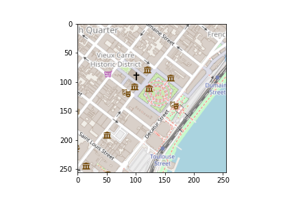
Producing a tile of Jackson Square in the French Quarter of New Orleans:
Stitching Tiles Together
To download all the tiles needed for our visual, we'll need to calculate the
limits of the data we'll be using in our visual. There are many ways we can do
this, all of them are valid. For simplicity though, I'll calculate the
min and max of both the lat and lon columns in
my pandas DataFrame:
top, bot = df.lat.max(), df.lat.min()
lef, rgt = df.lon.min(), df.lon.max()
This gives us a bounding box (in GPS coordinates) that encompasses our entire data-set.
Next, just like we did in the last section, we'll use
the point_to_pixels() function to convert our GPS coordinates into Web
Mercator coordinates.
zoom = 13
x0, y0 = point_to_pixels(lef, top, zoom)
x1, y1 = point_to_pixels(rgt, bot, zoom)
That we can then divide by TILE_SIZE to calculate the minimum and
maximum number of tiles we'll need to download for both the {x} and
{y} arguments for the API:
x0_tile, y0_tile = int(x0 / TILE_SIZE), int(y0 / TILE_SIZE)
x1_tile, y1_tile = math.ceil(x1 / TILE_SIZE), math.ceil(y1 / TILE_SIZE)
As a precaution, we'll add an assert statement to limit the number of
tiles we can download and save us from the embarrassment of accidentally
burdening OpenStreetMap tile servers.
assert (x1_tile - x0_tile) * (y1_tile - y0_tile) < 50, "That's too many tiles!"
Now that we've calculated which tiles we need to download from OpenStreetMap, we
can use the built-in itertools product() function
to loop through every tile, downloading and saving the tiles to a single large
pillow image using Pillow's paste() function:
from itertools import product

# full size image we'll add tiles to
img = Image.new('RGB', (
    (x1_tile - x0_tile) * TILE_SIZE,
    (y1_tile - y0_tile) * TILE_SIZE))

# loop through every tile inside our bounded box
for x_tile, y_tile in product(range(x0_tile, x1_tile), range(y0_tile, y1_tile)):
    with requests.get(URL(x=x_tile, y=y_tile, z=zoom)) as resp:
        resp.raise_for_status() # just in case
        tile_img = Image.open(BytesIO(resp.content))

    # add each tile to the full size image
    img.paste(
        im=tile_img,
        box=((x_tile - x0_tile) * TILE_SIZE, (y_tile - y0_tile) * TILE_SIZE))

plt.imshow(img)
plt.show()
Resulting in a plot like this:
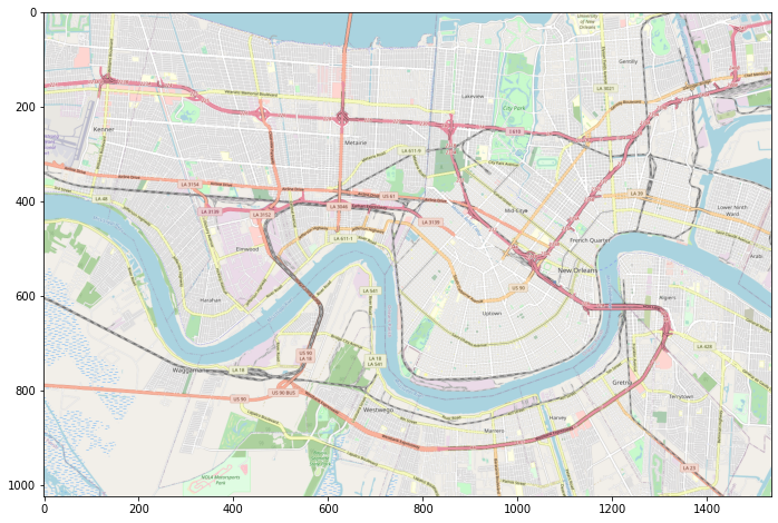
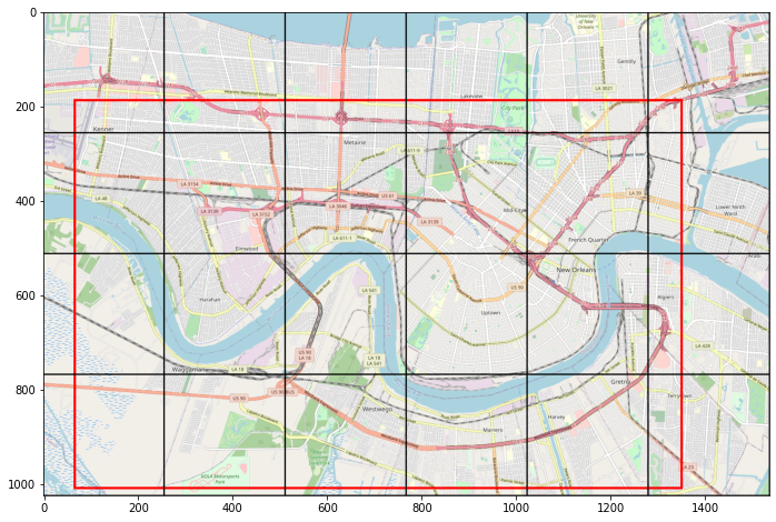
The eagle-eyed among us will notice the image is too large for the visual we
want to create. This is because of the math.ceil() and int()
functions we used to round the pixel coordinates into {x} and
{y} tiles we used above. To get our image back to size we'll need to
crop out the fractions of tiles not inside our bounding box.
Cropping the Basemap
To help my human-eyed brethren, I added some lines to our previous graphic to help understand what's going on. Essentially some fraction of each tile we've downloaded (outlined in black) will be used in our final visual (outlined in red) that we calculated in the last section. Our goal for this section is to trim the fraction of tiles outside of our red square.
To curtail our oversize image, we'll use pillow's Image.crop()
function, which takes a tuple (left, top, right, bottom) measured in
pixels from the top left corner to crop our image.
From our work above, we know the pixel
coordinates of the red square is defined as x0, y0 and x1, y1.
We can then multiply the tile coordinates x0_tile, y0_tile by
TILE_SIZE to find the pixel coordinates for the top-left corner of the
current (oversize) basemap:
x, y = x0_tile * TILE_SIZE, y0_tile * TILE_SIZE
Now it's just a simple process of subtracting the edges of our red square from the pixel coordinates we just calculated for our oversize image to crop it to our desired size:
img = img.crop((
    int(x - x0),  # left
    int(y - y0),  # top
    int(x - x1),  # right
    int(y - y1))) # bottom

plt.imshow(img)
plt.show()
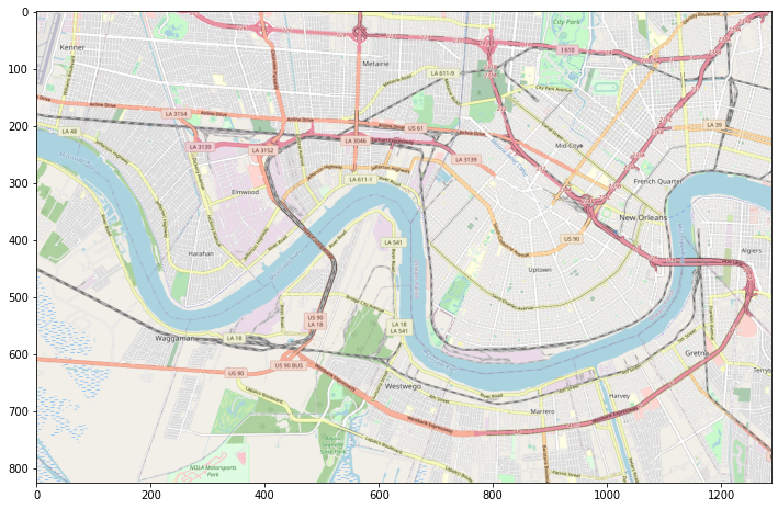
Resulting in our final (properly sized) basemap for our visual:
Plotting The Data
Finally, with our basemap created, we can plot our data just like any other
visual with some key exceptions. We can start by setting a matplotlib
subplots()
and a scatter()
plot for the lat and lon columns in our pandas DataFrames:
fig, ax = plt.subplots()
ax.scatter(df.lon, df.lat, alpha=0.1, c='red', s=1)
Then we'll add an extra argument to the imshow() function to properly
locate our image in the final visual. The extent argument is used to
move a image to a particular region in dataspace.
ax.imshow(img, extent=(lef, rgt, bot, top))
Next, we'll lock down the x and y axes to the limits we defined
a few sections ago by using the
set_ylim() and set_xlim() functions.
ax.set_ylim(bot, top)
ax.set_xlim(lef, rgt)
All of this work will produce a simple graphic with a (gorgeous) basemap of buses servicing New Orleans' Route 16.