You, Me & Machines... Learning
Developing our first neural network with Keras
In this essay, we’ll introduce the terms and how each component of a neural network works together to tackle a classic computer vision problem: analyze thousands of MNIST images of handwritten numbers and sort them (with 97.88% accuracy) into the digits they represent.

The Problem
For us, our brains have no trouble looking at low quality (28 by 28 pixel) images and deciphering their meaning. We’re essentially hardwired to find patterns in everything we see.

But how do we program a computer to do the same thing? Assuming there is no mathematical function we can use and a “6” can come in so many different shapes and forms, we can't rely on a specific part of an image to tell us what the number is.

This is where neural networks come to the rescue.
The idea behind modern neural networks, and all machine learning applications, is to analyze data and try to discover general patterns in that data so it can make predictions about new data it hasn't seen before. [1]
Meaning, we can use a neural network to let our computer discover the patterns in our images, and then use that pattern to sort each image into the digit it's depicting.
The Plan
So to solve our goal of accurately sorting images into the digits they represent, we’ll:
- Download and prepare thousands of images of hand written numbers.
- Build a feed forward neural network to analyze the images and sort them.
Then after we've built and trained the neural network to sort images for us:
- Test the neural network using another set of images it's never seen before to grade how well it classifies images.
First-up is preparing our computer to “learn."
Preparing The Environment
Before we get started, I should point out that I’ve published the jupyter notebooks I’ve used for writing this on a GitLab repository and Google Collab, so you can play with the code without installing anything on your computer.
If you want to set this up on your own computer, and you already have python installed, a simple pip command will install all the libraries we’ll need for this project.
$ pip install keras tensorflow numpy mnist
We’ll use TensorFlow (a powerful deep learning library published by Google) as a backend to Keras, a library that dramatically simplifies the programming required to build a neural network.
As per usual scientific and “big-math” related python projects, we’ll also need NumPy to give us fast multidimensional array support in python.
And finally we’ll utilize the MNIST dataset, which is a subset of a large database called the NIST Special Database. The MNIST dataset is maintained by Yann LeCun, contains the 70,000 images of handwritten numbers we’ll use to train and test our neural network.
Loading, & Exploring The Data
Now that we’ve built our working environment, we can download the images and begin preparing them for our neural network. Thankfully the MNIST library makes downloading thousands of images as simple as importing a module in a new python file.
import mnist

training_images = mnist.train_images()
training_labels = mnist.train_labels()

testing_images = mnist.test_images()
testing_labels = mnist.test_labels()
After the images have downloaded (could take a while on slower connections) we can see the MNIST library has helpfully put our images into a NumPy array for us.
print(type(training_images))  # <class 'numpy.ndarray'>
print(training_images.shape)  # (60000, 28, 28)
print(training_images.min())  # 0
print(training_images.max())  # 255
Printing out some statistics about our NumPy array tells us each image (60,000 images in the training set) is in a 28 by 28 pixel matrix, with each pixel having a value between 0 and 255 (an 8-bit number) to tell our computers how “on” that pixel should be. The higher the pixel’s value the more “on” that pixel will be.
And while this is great for our human eyes, this isn’t a great format for our neural network. Meaning, like all true data scientists, we have to massage some data.
Preparing The Data (Normalizing)
An important step in preparing our images for our neural network is to "normalize" them.
This (usually) speeds up the time it takes to train our neural network, as well as avoid any problems that arise, if we have multiple datasets that use different ranges.
For our images, we'll only need to scale their range from their current values [0 - 255] into a more standard range [0 - 1]. We can do this using a min-max feature scaling funciton:

And, because our minimum value is 0, we can simplify the formula to just dividing by our maximum value in our range (255).
# ensure our numpy arrays use floating point decimals
training_images = training_images.astype('float32')
testing_images = testing_images.astyle('float32')

# reduce range to [0 - 1] (normalize)
training_images = training_images / training_images.max()
testing_images = testing_images / testing_imaoges.max()
Reshaping our Data (Flattening)
Our neural network will expect each image to be in a long 1 dimensional list of pixels. This means we'll need to "flatten" our images by removing it's 2nd dimension before we can start training our neural network.
To “flatten” our images , we simply need to call NumPy’s reshape() method and specify a list of dimensions we want our new matrix in.
# flatten our images into 1 dimension
training_images = training_images.reshape((-1, 784))
testing_images = testing_images.reshape((-1, 784))
And just like that we’ve transformed our images from human readable to neural network readable.
# stats of our normalized data
print(training_images.shape)  # (60000, 784)
print(training_images.max()) # 1
print(training_images.min()) # 0
One-Hot Encoding
Now that we’ve finished preparing our images (questions) for our neural network, we can begin working on the labels (answers).
In order to train our neural network, we need to convert our labels from their perfectly human readable base-10 digit into a 10 item list format called “one-hot” encoding.

Without getting into too much detail, our neural network will have 10 output neurons with each neuron representing the probability of an image representing any digit in our 0-9 range.
We need to transform our labels into the probabilities that those 10 output neurons should output, effectively telling our neural network that we’re 100% sure this image is a 6.
To convert our labels into one-hot format, we need to use another NumPy method called eye()
# convert labels to ‘one-hot’ encoding
training_labels = np.eye(10)[training_labels]
testing_labels = np.eye(10)[testing_labels]
And with that, we’ve finished preparing our data to be processed by our neural network. Now’s the time to actually start building it.
Building The Model
The term “model” in machine learning has taken on a few different meanings from its original definition a few years ago [2]. In Keras, a model is used to describe the overall structure of our neural network.
There are two types of models we can build with Keras:
- We can define more complex networks using the Model API, which is more verbose (complex) when setting up, which could lead to errors if we’re not careful.
- Or we can use the Sequential API, which can only define a simple linear stack of layers, but makes up for this by removing a lot of the complexities the Model API has.
The type of neural network we’ll be building is called a feed-forward neural network. It’s essentially a single stack of layers, where each layer of neurons feeds their information forward to the next layer, making the Sequential API a perfect fit for our project.
from keras.models import Sequential
model = Sequential()
After we’ve initialized our Sequential model, we can use the model.add()
method to add individual layers to it later on.
Adding Layers
As you’ve probably gathered, a neural network is built by using many nodes called neurons.

Each input, in a neuron, is multiplied by a weight (importance factor) before being added together along with a bias. Then, to keep this number in a specific range, the number is then fed into an activation function (we'll learn about these later) to produce the neuron's output.

In a feed-forward neural network, neurons are organized into layers, where each neuron in a layer will only connect to the neurons from adjacent layers, forming a sequential stack of layers.

Typically each neuron in a layer will connect to every neuron from the adjacent layer, forming a fully interconnected (dense) layer of connections.

In Keras, we have many types of layers we can use in our model, however, for this project, we’ll only need to use the Dense layer.
from keras.layers import Dense
Layer No.1
For the first layer in our model, we'll be connecting the 784 neurons in our input layer (the pixels in our images) to the 512 neurons in our hidden layer.

To add a dense layer to our model, we simply need to initialize it with some
options, and add it to our model’s stack using the add() method we
talked about above.
model.add(Dense(512, activation='relu', input_shape=(784,)))
- The first argument, called units in the documentation, describes the number of neurons our hidden layer will have. 512 is a somewhat arbitrary decision I landed on while testing (playing around).
- Because this is the first layer in our stack, we need to tell Keras the input_shape our images will be in when we start training our neural network.
- The activation function, like we discussed, is how the neurons in our hidden layer will "squash" their outputs before outputting their results.
We’ll be using the Rectified Linear Units activation function (ReLU) which leaves any positive number unchanged but transforms any negative number into a 0 (no learning).

Layer No.2
Now that we’ve set up our first layer, we’ll need to build the connections to our output layer, allowing us to get the predictions out of our neural network.
Note
We can add more hidden layers here, but I found that having more than one did nothing to improve the accuracy of our neural network and slowed the learning rate considerably. Feel free to play around with my jupyter notebook to see what you find.
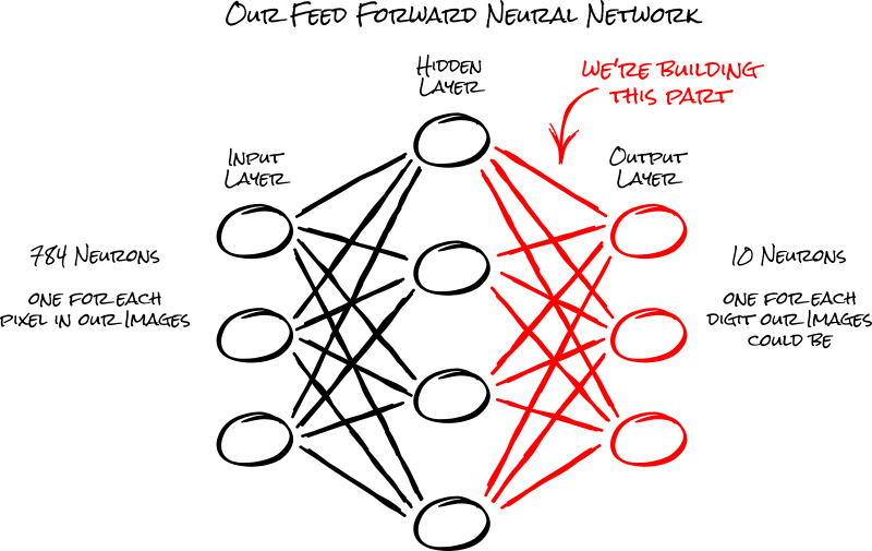
Our last Dense layer will be the output of our neural network. This layer will need 10 output neurons, one for each digit our image could be.
For the activation function, we'll use the softmax function, which allows us to calculate the activation of the 10 output neurons relative to each other. (eg: "I'm 20% sure this is a 4")

Also, because this is the second layer we're adding to our model, we can omit the input_shape argument we added in the first layer we built.
model.add(Dense(10, activation='softmax'))
And with that, thanks to the simplicity of Keras, we’ve finished building the structure of our neural network.
Compiling The Model
Now that we're done building the structure of our neural network, we can work on the methods and algorithms it will use to “learn” as we compile our neural network.
In Keras, we can simply call the model.compile() method with a couple of
options to prepare our neural network for service.
model.compile(
    loss='categorical_crossentropy',
    optimizer='adam',
    metrics=['accuracy'],
)
- The loss argument is telling Keras what type of loss function we want to use. A loss function is essentially a function used to measure how “wrong” our neural network is during training.
While Keras supports many types of loss functions, typically a loss function is chosen for us based on the decisions we've made eairler. For example, our neural network is classifying images, and we've encoded our labels into a "one-hot" format, meaning we need to use a categorical crossentropy loss function.
- The optimizer is a function used to adjust the weights and biases of our neurons in order to minimize the value of our loss function.
Much like with the loss function, Keras supports many types of optimizer functions. For our project, we’ll be using the ‘adam’ optimizer function, mainly because it’s usually a great optimizer.
- The metric argument tells Keras how we wish to evaluate how well our
neural network is doing. Usually this will be
metrics=[‘accuracy’]but for more complex networks with multiple output layers this can be different.
How To Train Your Model
Now that we have built the structure and defined how our neural network will “learn”, we can finally start the training process.
Training our neural network is easily done by calling the fit() method
as shown below, along with some extra arguments.
model.fit(
    training_images, # normalized images
    training_labels, # one-hot labels
    epochs=5,
    batch_size=64
)
The first 2 arguments are for our normalized and flattened images along with the one-hot encoded labels we’ll be using to train our neural network.
- The epochs argument tells Keras the number of times we will go through the entire set of images. Think of this as how many times you want to take the test.
- batch_size is the number of images our neural network should process before updating each neuron with the results from our optimizer function.
Note
Increasing the batch size is usually an acceptable tradeoff as it dramatically speeds up the learning process, with limited effects to overall accuracy. [3]
Running the model.fit() above will give us an output like this:
Epoch 1/5
60000/60000 [======] - 7s 118us/step - loss: 0.2309 - acc: 0.9330
Epoch 2/5
60000/60000 [======] - 7s 113us/step - loss: 0.0904 - acc: 0.9734
Epoch 3/5
60000/60000 [======] - 7s 114us/step - loss: 0.0588 - acc: 0.9824
Epoch 4/5
60000/60000 [======] - 7s 113us/step - loss: 0.0405 - acc: 0.9871
Epoch 5/5
60000/60000 [======] - 7s 114us/step - loss: 0.0302 - acc: 0.9908
Because we gave the metrics=[‘accuracy’] argument when we compiled the
neural network, acc: is printed in this output showing us how accurate
our neural network is after each epoch.
Looking at the last epoch, we can see our neural network achieved a 99.08% accuracy with our training data. Whoop!!!
But Wait! There's More!
Before we celebrate too hard though, keep in mind this score is from a test our neural network has already taken 5 times. Like aceing a test we’ve already taken, we can’t be sure if we just memorized the answer to the question, or really understood the material.
When our neural network is better at remembering answers than classifying images, it’s “overfitted,” [4] meaning it started using “patterns” in our data that doesn’t help it classify random handwritten numbers, but instead the specific handwritten numbers we gave it.
To determine if our neural network is overfitting, we’ll use the extra 10,000 images we prepared but we haven't given to our neural network yet.
The Ultimate Test
This time instead of calling fit() to train our neural network, we'll
call the evaluate() method to evaluate our neural network’s accuracy.
This time supplying the testing images and labels that our neural network
hasn't seen before.
This way, we can get an accuracy score on how well our neural network can sort any image of handwritten number, instead of just our dataset of handwritten numbers.
model.evaluate(
    testing_images,
    testing_labels,
    verbose=0
)
Running this code will give us the following output:
[0.07108291857463774, 0.9788]
- The first item in the array is the loss function value.
- The second item is our accuracy metric we asked for when we compiled the neural network above.
Meaning we’ve achieved a 97.88% accuracy score on fresh data!
Not bad for our first neural network.
More Reading:
| [1] | Approximation by Superpositions of a Sigmoidal Function - Cybenko, G. |
| [2] | Definition of "model" in machine learning - StackExchange |
| [3] | On Large-Batch Training for Deep Learning - Cornell University |
| [4] | The Definition of "overfiting" - Oxford Dictionaries |